Designing with Maps

When people talk about cartography—the process of making maps—they often call it “the intersection of science and art.”

Mapmakers, of course, want to create work that’s visually appealing and, yes, maybe even beautiful works of art. If you’re a designer, however, it’s not unreasonable for you to balk at the technology and precision of mapmaking.

Allow me to introduce a tool that helps you improve precision and accuracy in your mapmaking, while also allowing for your unique aesthetic creativity. I am the Lead Product Engineer for ArcGIS Maps for Adobe Creative Cloud, a relatively new mapmaking plug-in for Illustrator and Photoshop. This software gives you access to abundant and accurate map layers, both vector and raster.

We’ll be using the plug-in for Illustrator, which has become a celebrated cartography tool for many well-known and highly regarded mapping organizations. News media, local and national government agencies, as well as major mapmaking companies worldwide have all integrated Illustrator and the plug-in into their cartographic processes.

A Portal to Map Layers

A geographic information system, or GIS, is a database of data that is connected to a location. These troves of data are stored as vector and raster layers, all connected by location.

With Maps for Adobe Creative Cloud, users can add GIS layers to their maps in the plug-in, and download them as AI files, for impeccable design efficiency.

You can confidently create stunning and accurate maps at a precision level that makes sense for your projects, eliminating the need to tediously trace images or manually organize your map’s layers.

Get the Plug-in

ArcGIS Maps for Adobe Creative Cloud is developed by Esri, a leading GIS software systems company, and you can download it for macOS or Windows from esriurl.com/mapsforadobe. Once you install it, you can access the plug-in from the Window menu in Illustrator, where you will find it listed in the Extensions list along with your other installed plug-ins (Figure 1).

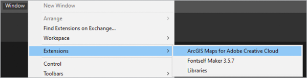
Figure 1. Open the plug-in from Illustrator’s Extensions list.

Open the plug-in to reach the sign-in screen, which offers three account options (Figure 2):

• ArcGIS Online and ArcGIS Enterprise: Most ArcGIS Online and ArcGIS Enterprise customers can log in to the plug-in with their ArcGIS Online sign-in credentials.
• Plus: This monthly subscription-based account offers most (but not all) Maps for Adobe Creative Cloud features. This category also offers a stripped-down Complimentary plan for non-commercial use.

Subscription pricing varies from $100–$500/year. For a full breakdown of the features available in each version, check out the Functionality Matrix and Pricing info.

For macOS users, the plug-in is Intel-based. Future releases will support the M1 chip natively; in the meantime, if you are using a M1-based machine, you will need to use the Intel version of Illustrator. Select the application icon, then go to File > Get Info and select Open Using Rosetta.

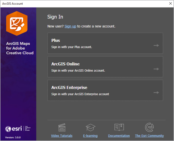
Figure 2. The plug-in sign-in screen shows three of the four account options.

Steps to Creating a Map

You can set yourself up with the plug-in to create a map in three steps:

1. Create a mapboard.
2. Add map layers.
3. Sync (download into Illustrator).

Of course, there is the magnificent fourth step, where you use your Illustrator skills and knowledge to apply your own unique graphic style and brand to your maps.

Preparing for precision

To demonstrate creating a map with ArcGIS Maps for Adobe Creative Cloud, I will focus on Bellingham Trails & Brew, a map of the trails, bike infrastructure, and breweries in my hometown.

My city sits along Washington’s Bellingham Bay and has an abundance of recreational trails. Bellingham also happens to have an abundance of craft breweries—among the highest per capita in the United States.

Because this is a city-level map, it requires a high level of precision, a mapmaking concept that deals with a map’s level of detail (see the sidebar, “Accuracy and Precision”).

Step 1: Create a Mapboard

In the plug-in, a mapboard represents the space on Earth that is mapped. In addition to spatial extent—the boundaries of your map that define its area—mapboards define the map’s name and scale. For my map I drew a large-scale (zoomed-in) mapboard over Bellingham, Washington.

To find Bellingham in the Mapboards panel basemap, I could have manually panned and zoomed to the desired location. Instead, I searched for Bellingham, Washington using the panel’s search feature (Figure 3), then selected my location from the list it returned. The basemap automatically zoomed to Bellingham.

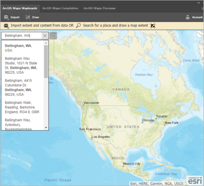
Figure 3. With a simple search, you can select from a list of geocoded locations to set the basemap.

I then used the plug-in’s Draw tool to create a rectangle over my desired map area to create my mapboard (Figure 4).

Configure your mapboard

The Mapboard Options dialog box automatically appears once you draw your mapboard, letting you configure your map name, size, and scale. Figure 5 (Next Page)shows the Mapboard Options settings for the Bellingham map. The available options are:

• Name: Here, you set the name of the AI file that the plug-in will create.
• Set Artboard Size: This section enables you to select from Illustrator preset sizes or to create a custom map size.
• Set Level of Detail: Select this option to lock in your map extent while also updating the scale. You can then adjust the size by adjusting the width and height values or by resizing the mapboard itself in the Mapboards panel.

There is direct relationship between any map’s extent, size, and scale. Note that adjusting the value of one of these three properties will change the other two settings.

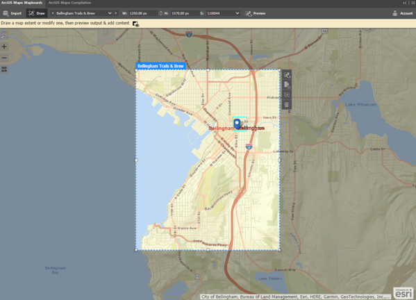
Figure 4. With the Mapboards panel basemap centered on the location, use the Draw tool to create a rectangle—your mapboard—over the desired map extent.

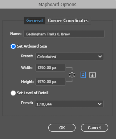
Figure 5. After you draw your mapboard, the Mapboard Options dialog box automatically appears.

Step 2: Add Map Layers

With a map’s extent and scale precisely set, the next step is to add layers to the mapboard in the Compilation panel.

To open the panel, click either of the two Preview buttons: the one in the Mapboards panel top bar or the other on the mapboard vertical toolbar (Figure 6).

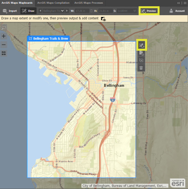
Figure 6. To add map layers, open the Compilation panel by clicking either of the preview buttons (highlighted).

Choose a new basemap (optional)

Basemaps are a collection of reference map features that provide readers with spatial context. Mapboards are automatically populated with a default basemap, which you can change.

For my map, I chose the World Navigation vector tile basemap (Figure 7).

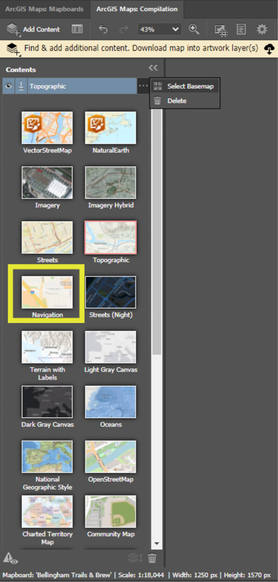
Figure 7. The Contents pane map gallery showing the Topographic vector tile basemap layer listed and the Navigation basemap highlighted

Esri’s vector tile basemaps are created from authoritative data sources and are regularly updated for accuracy. Each basemap varies in detail and design.

The World Navigation basemap includes highways, major roads, minor roads, railways, water features, cities, parks, landmarks, building footprints, and administrative boundaries. The presence and detail of each feature is determined by the map scale (zoom level) set in the Mapboard options.

To select a new basemap, click the more info (“meatball”) icon next to the name of the basemap layer and click Select Basemap to open the basemap gallery. Figure 8 shows the Compilation panel map preview area with the Navigation basemap added to the mapboard.

Note: When adding vector basemaps, only the name of the basemap is listed in the Contents pane, but all basemaps contain well-­organized map layers, including label layers.

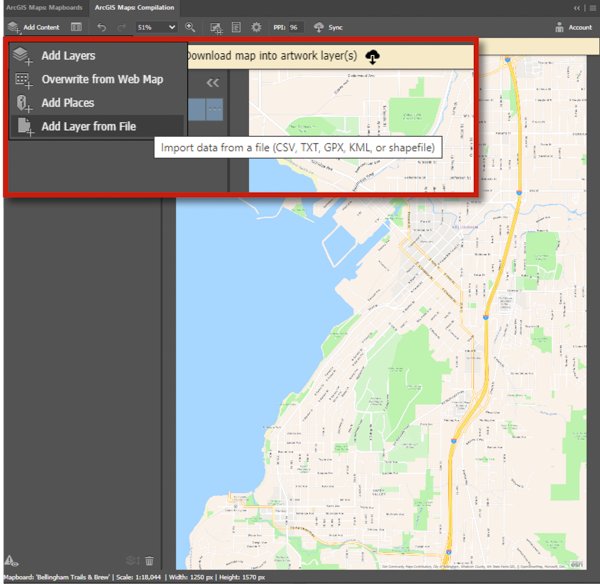
Figure 8. To add custom information to the map, select Add Content, then Add Layer from File.

Adding an individual layer

The Bellingham Trails & Brew map needed a single point for the precise location for each respective brewery. To add these, I added a custom point map layer CSV file (Figure 9). The most common way to add any map layer is from the Compilation panel. To do so, click Add Content, and select from the options:

• Add Layers: You can browse and add map layers hosted on ArcGIS Online.
• Overwrite from Web Map: You can add a web map, a collection of map layers hosted on ArcGIS Online.
• Add Places: You can search for specific places, like addresses, or multiple general locations, such as “university”, and add them to the map.
• Add Layer from File: You can add map layers from a local file on your computer. Supported file types are SHP, CSV, TXT, GPX, KML, and KMZ (see the sidebar, “A Designer’s Crash Course in Geographic File Types”).

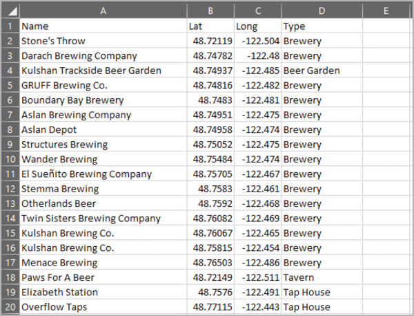
Figure 9. The CSV file with Bellingham brewery locations

In the CSV file for my brewery locations, the top header row contains the names for each point’s attributes. A point’s attributes can be anything that describes the spatial feature. For example, if your data features are the single locations (points) of beaches, their attributes could include any of the following—and much more:

• Ownership (public/private)
• Dogs allowed/not allowed
• Number of benches
• Tsunami threat rating
• Date the point was recorded in the database
• Cardinal facing direction (north/south/east/west)
• Shellfish collection permitted/not permitted
• Accessibility rating
• Number of boat launches

Below the headers, each subsequent row represents a single location (point) on the map, with data in each column defining the attributes of those locations.

For the plug-in to parse the file accurately and mark a precise location, your file needs a spatial attribute. For my large-scale (zoomed-in) map, the brewery locations require high precision, so I used latitude and longitude coordinates for my spatial attributes. For a map with less precise requirements, such as one that shows all major airports in the country, spatial attributes could include a column for city and a column for state.

Next, select Add Layer From File, locate the local file path to your CSV file (Bellingham_Breweries_2022.CSV, in my case), and open the file to instantly add your points to the map (Figure 10).

Figure 10. The map preview area shows the brewery point locations after adding the CSV file. The labels have also been added to these points.

Labeling map layers (optional)

Anyone who has made a map can appreciate the massive amount of time it takes to manually add labels one by one. Now with the plug-in, you can add map labels for entire layers with the click of a button.

To demonstrate this time-saving feature, I’ll show you how quickly I labeled the 19 breweries in my CSV layer.

First, I hovered the cursor over the Bellingham_Breweries_2022 layer’s More Options button to reveal the Layer Options menu. Then, I selected Manage Labels to add labels, which I further customized in the Label Configuration pane. Your options here are (Figure 11):

• Text: This menu lets you select the information from which labels can be generated. I selected my CSV file’s Name attribute. A menu lets you select a size range from 5 pt to 40 pt.
• Alignment: This option determines the label position in relation to the points.
• Show Overlapping Labels: The label visibility is determined by an algorithm that is optimized for interactive web maps, revealing labels on a hierarchical basis in a way that prevents overlapping. When you check this option, all labels will be visible and become part of the downloaded AI file.

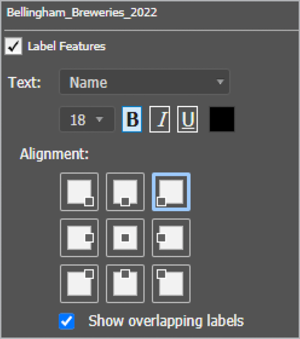
Figure 11. The Label Configuration pane in the Manage Labels dialog box

With the click of a button, I labeled the 19 points in my custom breweries layer automatically. Sometimes map layers can contain upwards of 100 features. Not only does the plug-in save time, it also ensures that each point is labeled correctly.

Adding a layer from the cloud (ArcGIS Online)

Because the World Navigation vector tile basemap is already rich with layers, I had only one more layer to add: Bellingham Neighborhoods.

Using Add Layers from the options, and then selecting the ArcGIS Online library in the Add Layers panel, I searched on the term Bellingham Neighborhoods from all content on ArcGIS Online (Figure 12).

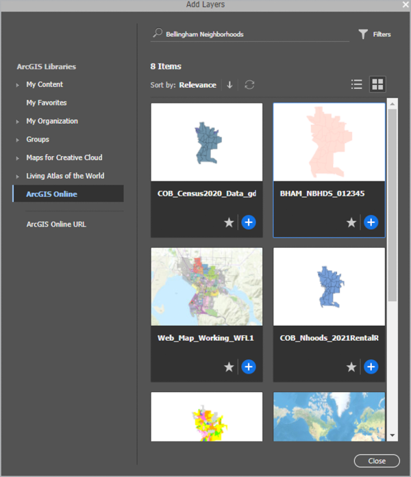
Figure 12. In the Add Layers panel, I search on the term Bellingham Neighborhoods from the ArcGIS Online library.

From the eight results, I added one layer that suited the map’s purpose, clicking the item’s plus (+) button.

The plug-in aligns the layer with those I previously added. To reorder the layers, I dragged the new layer beneath the Bellingham Breweries 2022 point layer (Figure 13). I also gave the new layer a custom name, Bellingham Neighborhoods.

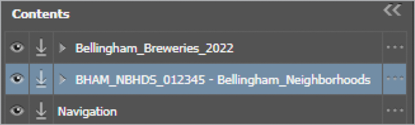
Figure 13. Drag the neighborhoods layer beneath the breweries layer to ensure the brewery locations are always visible.

Styling layers with the plug-in

Illustrator is a magnificent graphic design tool, but the plug-in has a few style options that can be useful in building your AI file.

For the example map, the new Bellingham Neighborhoods layer came with polygons (closed paths) defining each geographic area, each of which is filled by default. I wanted the neighborhood polygons to have only a stroke with no fill so that the layers beneath would be visible.

To adjust this, I first selected the Bellingham Neighborhoods layer in the Contents panel. I clicked the options button, then selected Change Style (Figure 14) to open the Styles options. Because I wanted all neighborhood polygons to be styled identically, I clicked Change Symbol Style from the options. From there, I set Fill to None. I then changed the stroke’s color and adjusted Line Width (Figure 15).

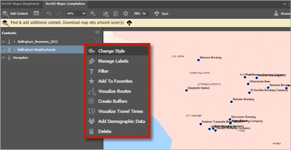
Figure 14. To change a layer’s style, open the layer options and select Change Style.

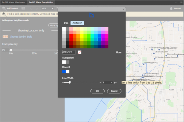
Figure 15. The Change Style options let me remove the fill color and set the stroke to blue, allowing the layers beneath the neighborhoods to be visible while displaying the neighborhood boundaries.

Adding raster data to a map

Because map readers may be interested to know where Bellingham’s hilly spots are, I added a raster layer to my map for a hillshade, which shows the shaded terrain relief of an area. Following the same steps as for the Bellingham Neighborhoods layer, I searched for hillshade in the ArcGIS Online library and selected Terrain: Multi-Directional Hillshade (Figure 16). The plug-in added this raster layer to my map and, just like before, perfectly aligned it with the other layers (Figure 17).

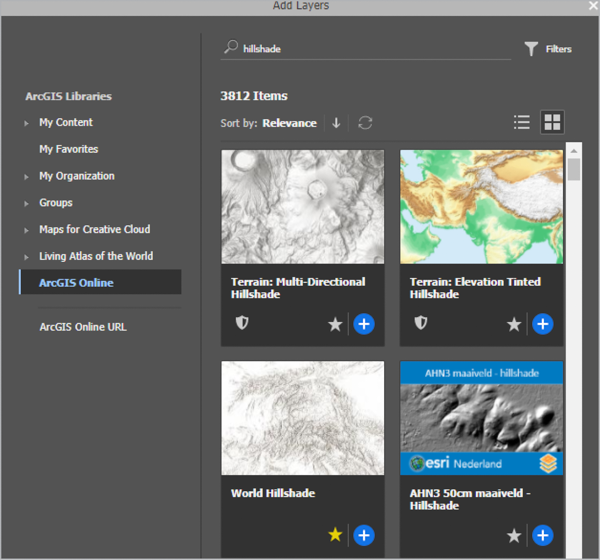
Figure 16. The Add Layers panel results after searching hillshade from the ArcGIS Online library

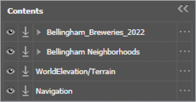
Figure 17. The Contents panel after adding the hillshade layer

Step 3: Sync (Download) the Map

After all your layers and labels are added, the moment has arrived: Create your AI file by clicking the Sync button on the Compilation panel’s horizontal toolbar. It might take a little time; how long depends on such factors as map size, feature detail, and internet speed.

For all paying plug-in users, the AI file remains synced to the plug-in, which means that you can always add more layers to the AI file at any time.

Map layers in Illustrator

After syncing, you can view your map as an AI file, with automatically organized layers (Figure 18).

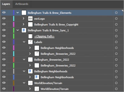
Figure 18. The organization for all the custom Bellingham Trails & Brew map labels and layers

The Bellingham Trails & Brew Sync_1 parent layer, for example, contains sublayers for all labels and all map features that Maps added in the first sync. A subsequent sync on this file would add a parent layer named Bellingham Trails & Brew Sync_2.

In Illustrator, the basemap parent layer name is World Navigation Map, as seen in Figure 19, and each sublayer contains either labels or map layers. Vector tile layers follow typical map organization. You’ll find the plug-in organizes labels at the top of the stack, followed by point layers, line layers and, finally, polygon layers.

Figure 19. Each sublayer within the World Navigation vector tile basemap organized by map feature

The World Navigation basemap’s design is clean and simple, which makes applying a unique aesthetic to the layers a breeze once the map is downloaded and you’re working on it in Illustrator.

Basemaps are tiled (split into sections) for optimal web display. As a result, vector tile basemap layers will be separated along this grid (Figure 20). Tiling does not impact the map’s appearance, but you may find the Illustrator Pathfinder Unite tool quite handy for uniting sliced polygons.

Take a look at the example map. Figure 21 shows the Illustrator artboard with all map layers visible except for the hillshade raster layer—just as it did in the Compilation panel map preview area.

Now the creative side of cartography can begin! Whether you are following the style guide of a client or you are applying your own unique aesthetic, you can now design the map’s look and feel around the well-organized cartographic underpinnings using Illustrator to create your final map project (Figure 22, next page).

You might notice that, in relation to Figure 21, Figure 22 is rotated. That is because Figure 22 was created with the previously mentioned ArcGIS Pro-to-Illustrator workflow, and I rotated the map in the process. However, in both figures, the map layers are identical, and therefore, except for the rotation, both looked identical prior to applying my own custom aesthetic in Illustrator. Here are some steps I performed in Illustrator to achieve my final map’s look.

The most noticeable change is the colors. Although the World Navigation tile basemap is wonderfully designed, I wanted my map to look unique. I also wanted the beer glass icons to pop out. For this reason, I greatly reduced the amount of colors in this map and made them quite subtle, minimizing saturation and value of each. To prevent visual overload, I removed the neighborhood borders altogether but kept their labels, spreading them over the extent of their respective areas. I placed the bike routes beneath the streets they follow, and then increased the routes’ width so that the street and routes were both visible. For the bike routes, I also chose brighter colors that contrasted with the overall palette of this map so that they would pop visually along with the beer glass icons.

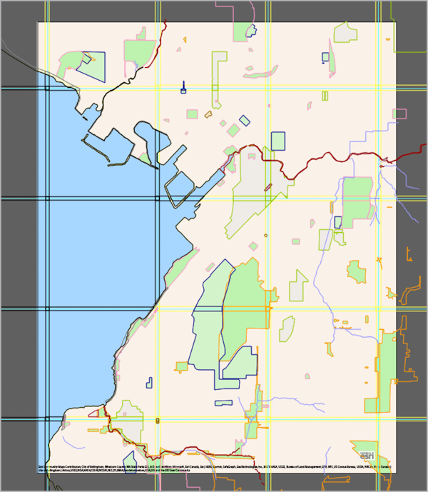
Figure 20. Vector tile basemaps will be sliced along their tile boundaries, as you can see when they are selected in Illustrator.

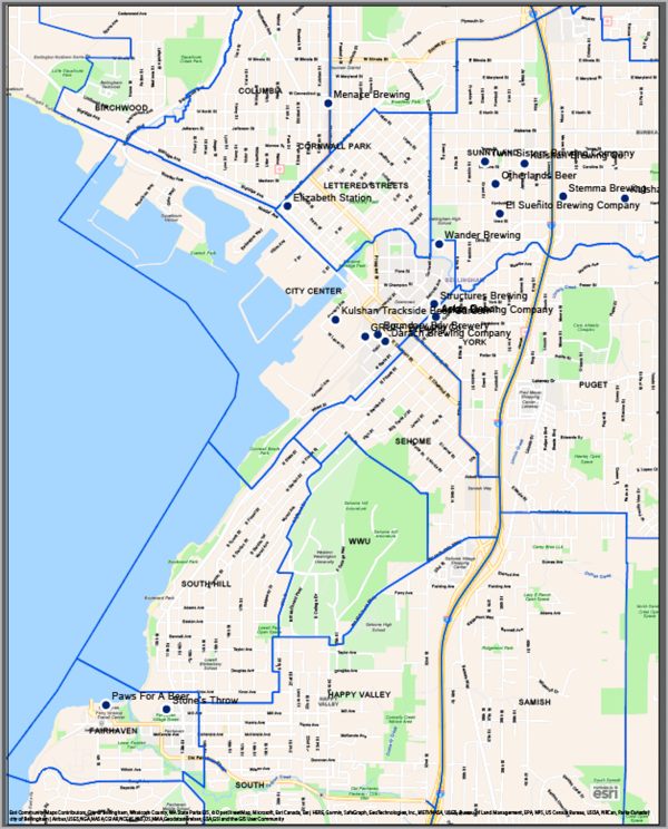
Figure 21. Your final Illustrator file will have the cartography organized and be all set for your creative touches.

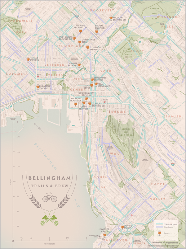
Figure 22. The Bellingham Trails & Brew map was made by Sarah Bell with ArcGIS Maps for Adobe Creative Cloud and Illustrator. In addition to the layers mentioned in this article, the final map includes a layer for the city of Bellingham’s bicycle infrastructure.

Mapping the Route to Great Design

With easy access to powerful and accurate map data, you can consider integrating accurate maps into all sorts of projects, like the beer can wrap in Figure 23. Have fun!

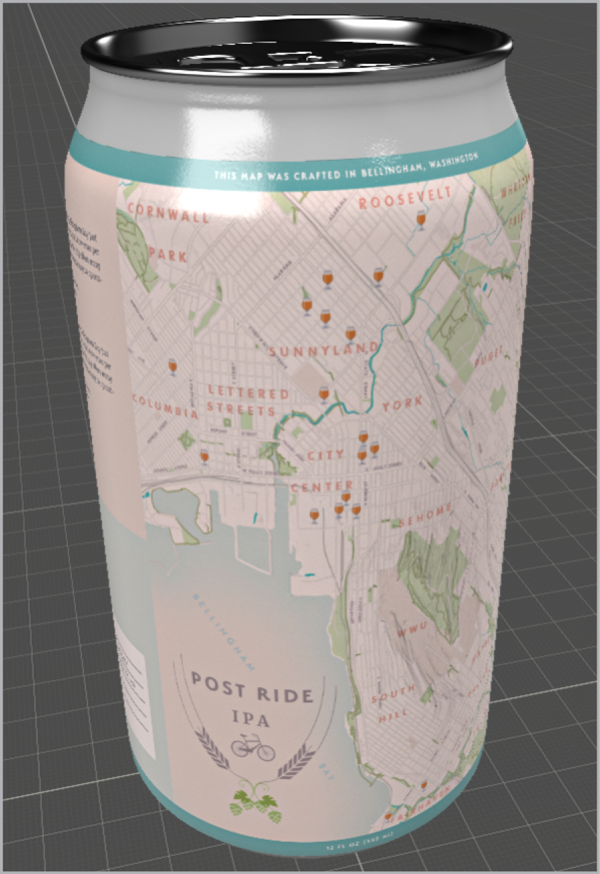
Figure 23. The map for this can wrap comes from the same map in Figure 22. It was simplified by the removal of several layers. The wrap was visualized in Adobe Dimension.