Excel for InDesign Users

Amazing Excel tips that will boost your page-layout productivity

I know it seems crazy to have an article about Excel in the middle of a magazine for Adobe InDesign users, but I’m serious: Learning a bit about Excel can really improve your productivity in the process of making books, catalogs, and all kinds of other layouts.

That’s because, every so often, you have a task in InDesign that could be handled easily with the data tools in Microsoft Excel. Maybe you need to clean up a bunch of text, or a table supplied by an author. Or your client or boss gave you an Excel document and wants you to turn it into something beautiful in InDesign. Believe me, the more you know about Excel, the happier you’ll be, no matter what you do!

In this article, I will show you how to use Excel and an amazing feature called Flash Fill (which was new in Excel 2013), plus some shortcuts for selecting large data sets and ways for comparing two lists.

Let’s start with some basic tips to help you navigate and manipulate your data in Excel. To follow along, download this file.

Shortcuts for Selecting Data

Even if you’re not a big fan of keyboard shortcuts, don’t skip this section. There are times when you really, really need them. For example, let’s say a client just sent you 5,000 rows of data in Excel. You need to quickly select from row 2 down to the end of the data. Using the PageDown key will take forever. Fortunately, there is a faster way: Pressing Command/Ctrl plus an arrow key (on your keyboard) is a fast way to jump to the edge of a data set. Or, if

you are already at the edge of a data set, the same command (Command/Ctrl plus an arrow key) will jump a gap (a column or row of empty cells) to move to the next data set.

Consider Figure 1. You have headings in row 1 and labels in column A. There are hundreds of rows of data filling columns B through F. Over in column I, there are some extra notes. The active cell is currently B2.

Figure 1.

• From cell B2, pressing Command/Ctrl + Right Arrow will jump to F2.
• From cell F2, pressing Command/Ctrl + Right Arrow again will jump the gap and land on cell I2.
• From cell B2, pressing Command/Ctrl + Down Arrow will jump to cell B700.
• From cell B700, pressing Command/Ctrl + Right Arrow will jump to cell F700.
• From cell F700 pressing Command/Ctrl + Right Arrow will jump to the right edge of Excel: XFD700. By the way, if you have data way out here, you have bigger problems than just learning the shortcuts. Just remember you can always press Command/Ctrl + Home to get you back to a safe familiar place.

Now here’s the cool part: Add the Shift key to any of the above to select from the current cell to the edge of the data (Figure 2). So, for example, starting from cell B2, press Command/Ctrl + Shift + Down Arrow and then Command/Ctrl + Shift + Right Arrow to select all the cells from B2:F700. You can then perform any formatting, such as increasing decimals or adding a thousands separator (both tools are found in the Home tab of the ribbon).

Figure 2.

Note: If you don’t mind including the headings in your selection, pressing Command/Ctrl + A selects what Excel calls the Current Region. From D6, pressing Command/Ctrl + A would select A1 to F700. The notes in column I would not be included because cells G1:G700 are empty.

Quickly Converting Date Format

Does 01/07/2019 mean January 7 or July 1? If your data is crossing between Europe and North America, it can be hard to tell. Excel only handles the conversion for you when the data is truly stored in your worksheet as dates. If the data arrives as text, then expect a disaster that will need to be cleaned up.

Fortunately, we’ve got some cleanup tips. In Figure 3, Excel did not understand that 20191115 meant November 15, 2019, and so the data was imported as text.

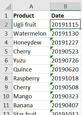
Figure 3.

To convert the text dates to real dates, follow these steps:

 1. From cell B2, press Command/Ctrl + Shift + Down Arrow to select all of the dates in column B. 2. On the Data tab, choose Text to Columns. 3. In the Convert Text to Columns Wizard Step 1, choose Fixed Width. Click Next (Figure 4).

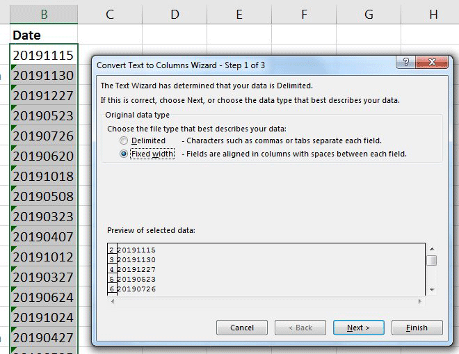
Figure 4.

In Step 2 of the Wizard, you should expect to see no vertical lines in the preview window (Figure 5). If a line appears, double-click the line to remove it per the instructions at the top of the wizard. Although this feature is called Text to Columns, your goal is to not actually split this text into multiple columns; you are simply trying to get to the formatting tools in step 3 of the Wizard.

Figure 5.

 5. In Step 3 of the wizard, choose Date as the data type. Open the drop-down menu, and choose YMD, indicating that your dates are in Year, Month, Day sequence (Figure 6).

Figure 6.

 6. Click Finish to return to Excel. Your text dates will be real dates.

 7. Finally, if you need to change the format of the date (so it looks like a date in the cell), press Command/Ctrl + 1 to display the Format Cells dialog box. By default, Excel should show you the Number tab and have pre-selected the Date category on the right. Choose any available number format (Figure 7).

Figure 7.

Joining Columns Using a Formula

Those data geeks in the I.T. department love to store first name and last name in two different fields. You, being a human, prefer to have the name all in one column. And you, the human, are now in charge of this file, so you want to have it your way. There are a few ways to fix this. Let’s start with a simple formula.

Remember that all formulas in Excel must start with an equals sign, but be aware that simple formula techniques you may be familiar with for number operations don’t work for text. And you might try to use plus symbols to add two cells together, but that also won’t work for text. Instead, use an ampersand.

In Figure 8, =A2&B2&C2 smashes all of the data from columns A, B, and C into a single column. It’s a nice first step, but, clearly, that’s all it is.

Figure 8.

Let’s add some spaces and a dot: You can concatenate cell values with literals in quotation marks. So, this code looks better: =A2&” “&B2&”. “&C2 (Figure 9).

Figure 9.

Next, to convert from upper case to proper case (what you might call Title Case), use the PROPER() function: =PROPER(A2&” “&B2&”. “&C2). In case you are wondering, =UPPER() converts to uppercase and =LOWER() converts to lowercase.

Now that you have the perfect formula in D2, select that cell, and double-click the fill handle to quickly copy the formula down. The fill handle is the square dot in the lower right corner of the active cell (Figure 10).

Figure 10.

Note: Double-clicking the fill handle only works if there are no blank rows in the data to the left. A blank row will fool Excel and cause the formula to stop copying right at the blank row. If you have data separated by blank rows, it might be easier to drag the fill handle down to the last row instead of double-clicking.

Caution: Now that you have a full name in column D, don’t delete columns A, B, and C yet! First you need to convert your formulas in column D to values:

 1. Select the data in column D. Start in D2. Press Command/Ctrl + Shift + Down Arrow.

 2. Press Command/Ctrl + C to copy.

 3. Click the small arrow on the Paste icon on the Home tab to reveal a number of Paste options (Figure 11), and choose Paste Values. (Alternatively, on a Mac you can choose Edit > Paste Special, and then choose Values.)

Figure 11.

Joining Columns Using Flash Fill

Formulas aren’t the only tool for merging the content of multiple columns; I’m happy to say, there’s also Flash Fill. Introduced in Excel 2013 (Windows) and Excel 2016 (Mac), Flash Fill is a magical feature that eliminates the need to know obscure Excel formulas. You simply type a few examples of what you want and ask Excel to follow your examples.

Note: In order for Flash Fill to work, all your columns must have a one-row heading. If your data does not have a heading, insert a new row above the data, and type fake headings to allow Flash Fill to work.

Once again, let’s use the same worksheet with people’s names in it. Say that you wanted to show last name followed by both initials in column D. First, type a few examples of how you want the data to appear. Sometimes, one example is enough. But if the single example is ambiguous, type a few extra examples.

Select the blank cell below your examples, and then press Command/Ctrl + E or click Flash Fill in the Data tab (Figure 12).

Figure 12.

Excel detects the pattern and fills in the rest of the column (Figure 13).

Figure 13.

Flash Fill is amazing, but not perfect

Always carefully study the results of Flash Fill. Excel is looking for any pattern, and it might use a pattern that makes sense to its computer-brain, but does not make sense to humans. For example, say that you only used a single example of Albert, P. A. before invoking Flash Fill. You and I would guess that you meant “Last Name, Comma, Space, First Initial, Period, Space, Middle Initial, Period” (Figure 14).

Figure 14.

But Excel sees a different pattern. It thinks that you want to replace the first letter of column D with the initial from column C, add a comma, space, first initial from column B, period, space, and then re-use the initial from C. This leads to a comical disaster, such as Lorna V. Banuilos becoming Vanuilos (Figure 15).  Oops.

Figure 15.

Fortunately, the fix is easy: press Command/Ctrl + Z to undo, type one or two more examples for it to learn the pattern you want, and try Flash Fill again.

Teaching Flash Fill two rules

Sometimes, when you’re using Flash Fill to clean up data, you’ll find it requires two steps. For example, in Figure 16, you’ve set up an example that shows the middle initial followed by a space.

Figure 16.

But what about names that don’t include a middle initial? After choosing Flash Fill, you see the extra period that appears when someone does not have a middle initial (Figure 17).

Figure 17.

Here’s the good news: Immediately after you perform a Flash Fill, Excel is waiting for you to make a correction. So you can edit Zack in cell E3, taking out the dot and extra space. As you edit, an outline may appear around E3:E12 to indicate that Flash Fill is ready to learn the second rule (Figure 18).

Figure 18.

Now, when you press Enter to accept the corrected entry, Flash Fill will look for other examples that it can change (Figure 19).

Figure 19.

The status bar in the lower left corner of Excel reports how many additional cells Flash Fill changed to fit the new rule. A Flash Fill icon appears near the range with options to accept the changes or to select the changed cells so you can tab between them (Figure 20).

Figure 20.

Using Flash Fill to extract data from a column

Flash Fill can also extract data from a cell that contains multiple fields. In the following example, column A contains a movie title, release year, and genre. This is an example where Text to Columns would fail—the genre would end up in column F for row 2 and column C for row 3. Flash Fill works perfectly to get the title, year, or genre. Just add a new column (don’t forget the header!), and type a couple of genres, so Excel sees the pattern (Figure 21).

Figure 21.

Now, select cell B4, and press Command/Ctrl + E. Flash Fill fills in the rest of the genres for you (Figure 22)!

Figure 22.

Preventing Flash Fill from Happening Automatically

By default, on Windows, Flash Fill is set to happen automatically. If you type Sci-Fi in B2 and start to type C for Comedy in B3, Flash Fill would “grey in” a suggestion of what it would like to do. This might be great for allowing people to discover Flash Fill. But now that you understand how Flash Fill can fail with ambiguous data, you might want to type more than one example before invoking Flash Fill. So, I always go to File > Options > Advanced and turn off Automatically Flash Fill (Figure 23).

Figure 23.

Excel for Mac doesn’t appear to have this Auto feature.

Comparing Two Lists

Your deadline is tomorrow. The client just sent an updated data file in Excel. Did they mark the changes in red? Of course not! So how can you find out quickly what changed?

There are three common methods for comparing two sets of data:

• Use VLOOKUP in both lists
• Use MATCH in both lists
• Combine all of the lists and use a pivot table

Using MATCH or VLOOKUP

The MATCH function in Excel answers the question “is something there in the other list?” For example, let’s look at Figure 24A. I have two lists—one in column A and one in column D—and I want to find out if the values in the second list exist in the first one.

Figure 24a.

So, in cell E2, the formula =MATCH(D2,$A$2:$A$23,0) (Figure 24B) means: look for the value in D2 inside the range between A2 and A23—and if “Apple” is found in column A, then return a number, and if not, then return an error (“#N/A”).

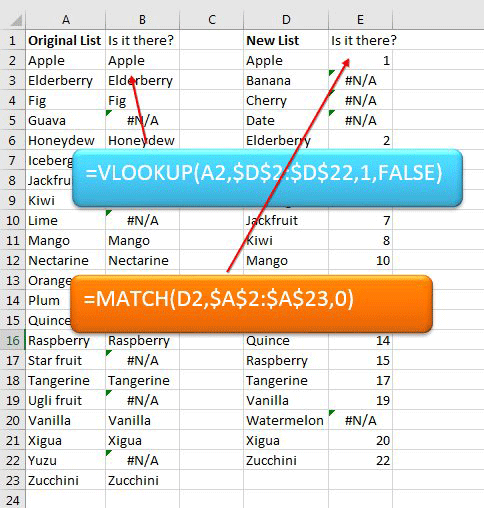
Figure 24b.

The 1 you see in the Figure 24C, means that “Apple” is the first item in the range A2:A23. Note that I almost never need to know where exactly something is—I just need to know if it is in the other list. When I look at all the results in column E, I see the #N/A to mean the item is missing from the first list, and every other answer means “it is there.”

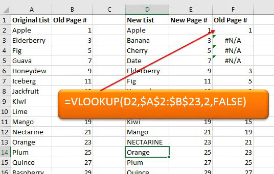
Figure 24c.

TIP: When you’re typing a formula, you can press F4 to add the $ symbols for you. (This shortcut was added in Excel 2016 for Mac.)

In Figure 24B, you can also see a VLOOKUP formula, which does something similar. In this case, the arguments (the stuff inside the parentheses) are similar to the MATCH but sort of in reverse—they mean “look for the term found in cell A2 in the range of cells between D2 and D22.” But there is an extra, third argument in VLOOKUP to indicate which column of the lookup table to return. The result is that it returns “Apple” instead of just the number 1. But again, in either case, I only care about the #N/A errors—the ones that say this term is not in that other list.

Why do people prefer VLOOKUP to MATCH? Because VLOOKUP can return something from a matching row. For example, in Figure 24C, we have added a column of page numbers, like from an index. The VLOOKUP formula in column F tells you not just if the index entry was found, but also what page number it was originally found on! The third argument here tells you which column from the first list to return (in this case, the second column).

Is this complex? Sure, at first! But after you try it a few times, it’s like being given a new superpower.

Using a pivot table to compare two (or more) lists

The methods above work fine and I have used them thousands of times. But I am fully aware that VLOOKUP is a scary concept to someone who uses Excel infrequently. (It is only a rumor that Microsoft will send you a vinyl pocket protector with the word “NERD” on it if you mention VLOOKUP to your friends at a party.)

So if you think VLOOKUP is a big ugly hairy scary monster, let me offer you an alternative which is only a medium-sized ugly scruffy monster: a pivot table. I can already see your reaction, because I’ve seen it hundreds of times. You have both hands up, you are backing away from your tablet, and you are saying, “no, no, I am really sure I don’t need a pivot table….”  But I think you’ll find that comparing two lists is dramatically easier with a pivot table.

Let me walk you through it in a few steps. Let’s go back to your original list of produce.

Add a blank column to the right of your original list (Figure 25).

Figure 25.

Type the heading “Source.” Select B2:B17. Type Original, and press Command/Ctrl + Enter to enter the word Original in all of the selected cells. Change the heading in A1 to Product  (Figure 26).

Figure 26.

Use Command/Ctrl + X to cut D2:D16 to the clipboard. Select A18, and press Command/Ctrl + V to paste.

Select B18:B32. Type “New,” and then press Command/Ctrl + Enter to fill that range with the word New. So you end up with just two columns: the first one with the combined list of products from the original two columns, and the second one with the source of those items “original” or “new” (Figure 27).

Figure 27.

After that tiny bit of pre-work, you have the pieces to create the pivot table.

Select one cell in your data. Any one cell. Don’t select two cells!

From the Insert tab, choose PivotTable. The Create PivotTable dialog box appears.

Most of the settings will be correct. Change from New Worksheet to Existing Worksheet. Click in the blank field, and then click in a blank section of your worksheet (I used F2 in Figure 28).

Figure 28.

Click OK.

Excel displays the PivotTable Fields panel.

Drag Product from the top of the panel down into the Rows area. Drag Source to the Columns area. Drag Product (again) to the Values area. Your panel should look like Figure 29.

Figure 29.

The resulting pivot table will look like Figure 30.

Figure 30.

Any zero (or blank space) in the pivot table indicates a problem or a mismatch. For example, Cherry and Date are in the new list but missing from the original list. Fig and Guava are in the original list but missing from the new list.

Once again, this is one of those Excel features that is overwhelming the first time you encounter it, but is actually easily manageable if you follow the rules and try it several times.

Faster Ways to Filter

The more data you have, the harder it is to find just what you’re looking for. Excel is great at sorting your data, of course, but another option is filtering—where you can sort all the data and then tell Excel what to display and what not to. Filtering is really easy to do, but there’s a fast way to filter and a slow way. Unfortunately, most Excel users have only discovered the slow way!

In case you’re not familiar with filtering, I’ll show you the “long way” first (as it helps you understand all the moving parts). Then I’ll show you the fast way.

 1. First, choose any one cell in your data.

 2. Go to the Data tab of the ribbon, find the big Filter icon, and click it (Figure 31).

Figure 31.

You now have a filter drop-down menu attached to each heading (top row) in your data (Figure 32).

Figure 32.

 3. When you click one of the little drop-down (down arrow) icons in the header, you can see the filter options. In Figure 32, you can see the Filter drop-down menu for “Rep.”

 4. At the bottom of the filter options you’ll see a list of all the different data in that column, automatically sorted (even if the data itself isn’t sorted). By default, ever since Excel 2007, every item is pre-selected. So, to choose a single rep, you have to uncheck Select All (Figure 33).

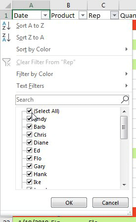
Figure 33.

 5. After deselecting Select All, you then scroll to find the item you’re interested in, and choose it. In this figure, I am selecting Will (Figure 34).

Figure 34.

That seems simple enough. Let’s count the clicks: Select One Cell, Data, Filter, Drop-down, Uncheck Select All, Scroll, Scroll Some More, Will, OK. Only eight or nine clicks, depending on how many times you clicked below the scroll bar to page through. Nine clicks. How can you make that easier?

The faster way: filter by selection

Believe me, there is a much easier way to filter. Spend 60 seconds now, and your life will be faster every time you open Excel to create an ad hoc selection.

Say that you need to find all of the watermelon sales. Open the Excel workbook. Scan through the product column, and select a cell that says Watermelon. All you need to do is right-click on that cell, and then choose Filter > Filter by Selected Cell’s Value.

Two clicks. That’s it. You now have all of the watermelon records. That was so easy; let’s take it up one notch. Let’s say that you now need only the Zeke sales of watermelons. Right-click any cell that contains Zeke, and choose that same feature from the context menu (Figure 35).

Figure 35.

You now have just the five records where Zeke sold watermelons (Figure 36). All in just a couple of clicks!

Figure 36.

I should point out that in Excel for Windows you can make this process even faster and easier by adding something called the AutoFilter to the Quick Access Toolbar. I’m not sure why this awesome feature isn’t available on the Mac, but maybe it will be in the future. If you’re a Windows user, check out my article about AutoFilter here on my site.

Seeing Totals of Only the Visible Cells

While we are talking about filters, here is another cool trick that most Excel users haven’t learned yet. After applying a filter, you can create a subtotal beneath a column, and that subtotal will change automatically when you change the filter setting. Here’s how it works: Once you’ve applied a filter, go to the first blank row below your data. Select one or more blank cells below the numeric columns (this only works for columns with numbers), and click the AutoSum button in the Home or Formulas tab.

Normally, AutoSum gives you a SUM function in the cell. But because you are below a filtered data set, Excel inserts a SUBTOTAL function instead. This formula adds only the rows you can see (Figure 37).

Figure 37.

Now, you can click the Filter button at the top of the column and turn on and off checkboxes to add or remove from the filtered list(Figure 38).

Figure 38.

After changing the filter selections, your subtotal formula updates.

Filtering by color

As an accountant, I love to mark records by putting an “x” out to the right of the data. But my creative friends love to mark records by turning the fill color green or magenta or cyan. They then want to filter by just the colored cells. Thankfully, Excel has sort and filter options for this, too.

If you need to see all the green cells, right-click any cell that is green. From the context menu that appears, choose Filter > By Selected Cell’s Color (Figure 39).

Figure 39.

(Or, if your manager marked cells by changing the text to red, you can choose By Selected Cell’s Font Color.)

The result: you will see only the green rows (Figure 40).

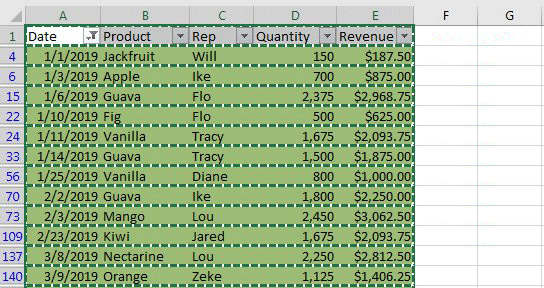
Figure 40.

Another trick: Select all of the data in the visible cells by pressing Command/Ctrl + A. Then you can copy them all with Command/Ctrl + C. When you paste to a new worksheet, you will get only the visible cells.

InDesign versus Excel

Alright … show of hands: would you rather spend a day in InDesign or a day in Excel? The vote totals will be 99999 to 1. And that’s only because they let me cast a vote (Figure 41).

Figure 41.

I get it: Excel is intimidating if you don’t spend 40 hours a week there. If it helps, I am just as intimidated by InDesign as you are intimidated by Excel.

If you’ve read this far, you are now aware of several powerful and empowering facts:

• There are faster ways to select data in Excel.
• Flash Fill will break data apart or join other data back together without writing a formula.
• When you’ve got to compare lists, pivot tables are likely to be a lesser monster than VLOOKUP.
• Finally, you have some filtering tricks even when your manager marked all the desired cells in green.